Imager as image editor
Simon Barthelmé (GIPSA-lab, CNRS)
Many people will be familiar with the set of tools available in Photoshop and the Gimp (various forms of selections, brushes, erasers, etc.). Here’s a screenshot of what the Gimp has to offer:
gimp-toolbox-icons.png
The goal of this document is to show how to perform most of these operations in imager, with the help of a few other packages. It’s a good way of familiarising yourself with the package.
library(imager)
parrots <- load.example("parrots")
1 Selection
1.1 Colour picker
This tool looks up the colour value at a certain location: in imager,
color.at(parrots,230,30)[1] 0.3098039 0.3058824 0.2196078You can also try grabPoint, which is interactive.
1.2 Rectangular selections
To directly obtain a rectangular image subset use imsub:
#A rectangular selection from (10,30) to (150,100)
imsub(parrots,x %inr% c(30,150),y %inr% c(10,100)) %>% plot
If what you need is a pixset, here’s a way:
px <- (Xc(parrots) %inr% c(30,150)) & (Yc(parrots) %inr% c(10,100))
plot(parrots)
highlight(px)
There’s also a function to do this interactively called “grabRect”.
1.3 Circular/elliptical selections
Use coordinates and the equation for a circle:
plot(parrots)
px <- (Xc(parrots) - 200)^2 + (Yc(parrots) - 350)^2 < 150^2
highlight(px)
Similarly, you can use an elliptical equation to select an ellipse:
plot(parrots)
px <- ((Xc(parrots) - 200)/3)^2 + (Yc(parrots) - 350)^2 < 150^2
highlight(px)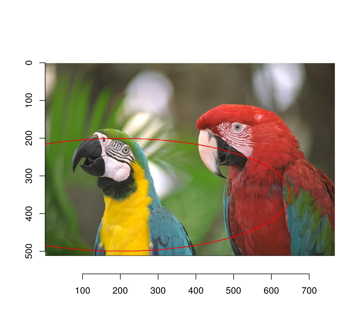
A change of coordinates is often useful: here we select a circle centered at the center of the image
#Define a new coordinate system with 0 at the center of the image
Xcc <- function(im) Xc(im) - width(im)/2
Ycc <- function(im) Yc(im) - height(im)/2
px <- (Xcc(parrots)^2+Ycc(parrots)^2) < 100^2
plot(parrots)
highlight(px)
1.4 Image color at a point
Use color.at:
color.at(parrots,24,55)[1] 0.5647059 0.5568627 0.40392161.5 Selection by similarity
For grayscale images this is easy: we want the set of locations \(x,y\), such that
\[ \vert I(x,y) - c \vert < \eps \]
where \(c\) is our target grayscale level, and \(\eps\) is a tolerance. We begin by computing the difference to the target:
boats.gs <- grayscale(boats)
val <- at(boats.gs,180,216) #Grab pixel value at coord (240,220)
D <- abs(boats.gs-val) #A difference map
plot(D,main="Difference to target value")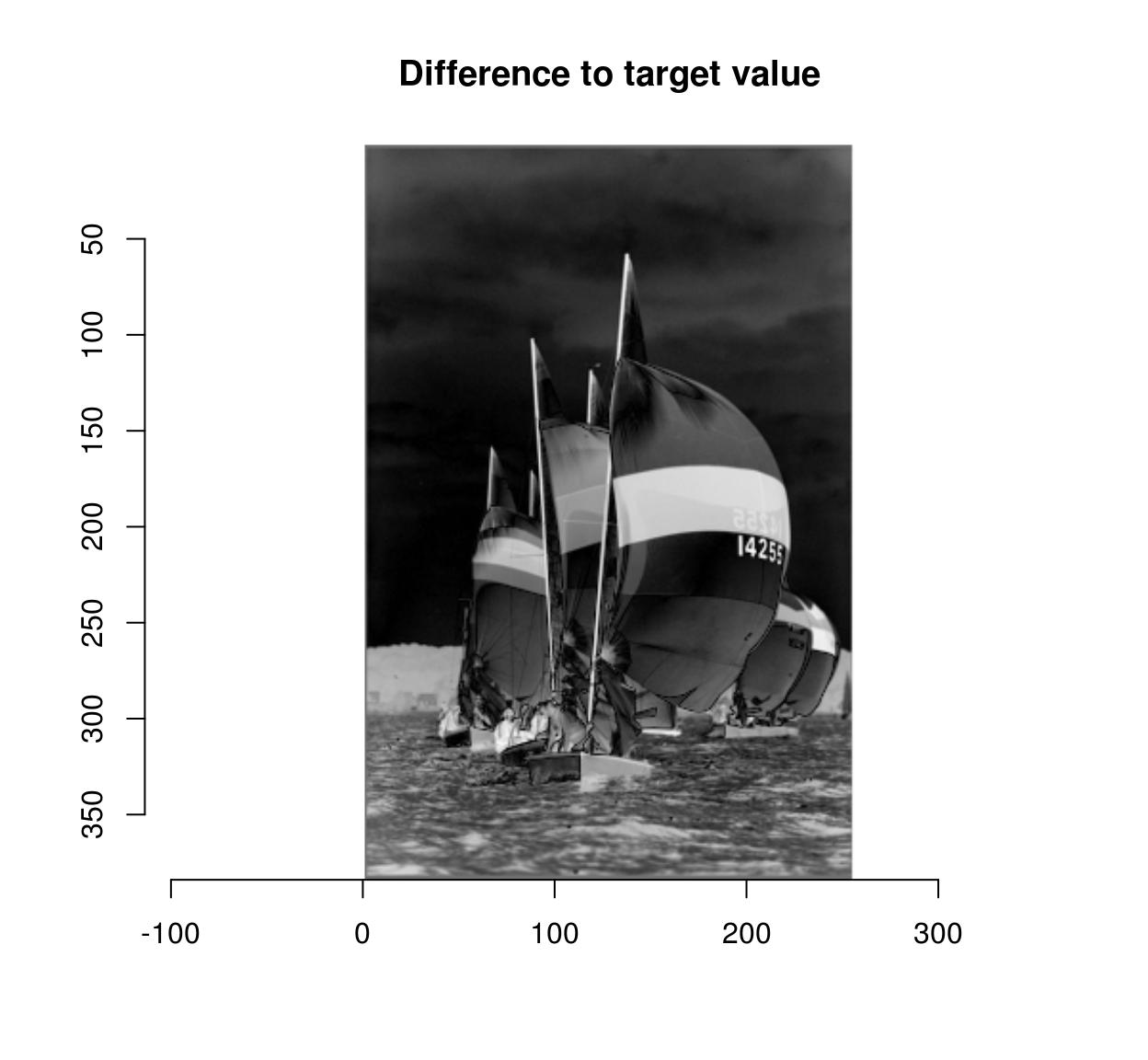
The distance map can then be thresholded to yield a pixel set:
plot(boats.gs)
highlight(D < .05) # epsilon = .05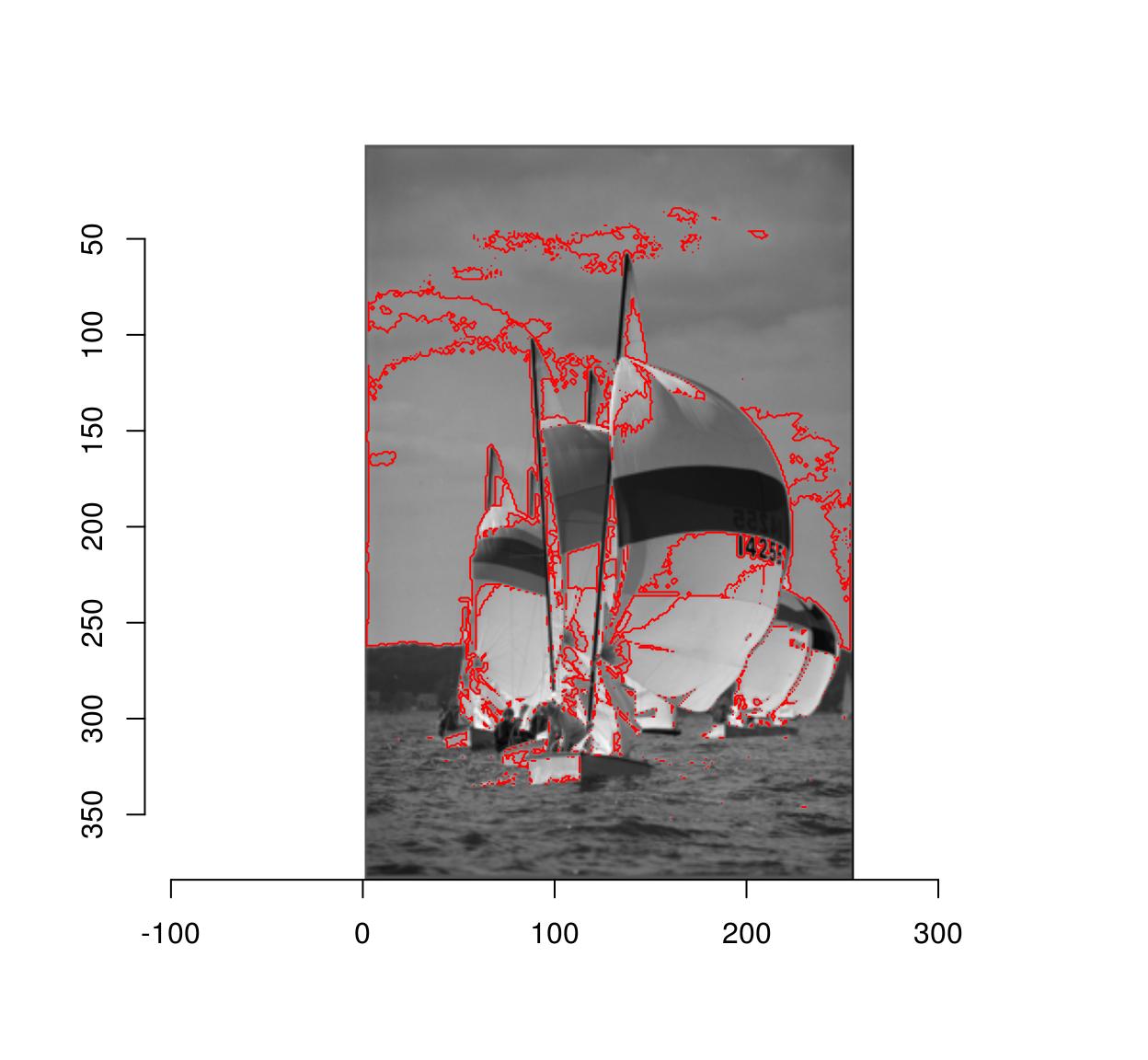
Due to noise the regions may be very irregular. Better results can often be obtained using smoothing:
plot(boats.gs)
isoblur(boats.gs,2) %>% { abs(. - val) < .05 } %>% highlight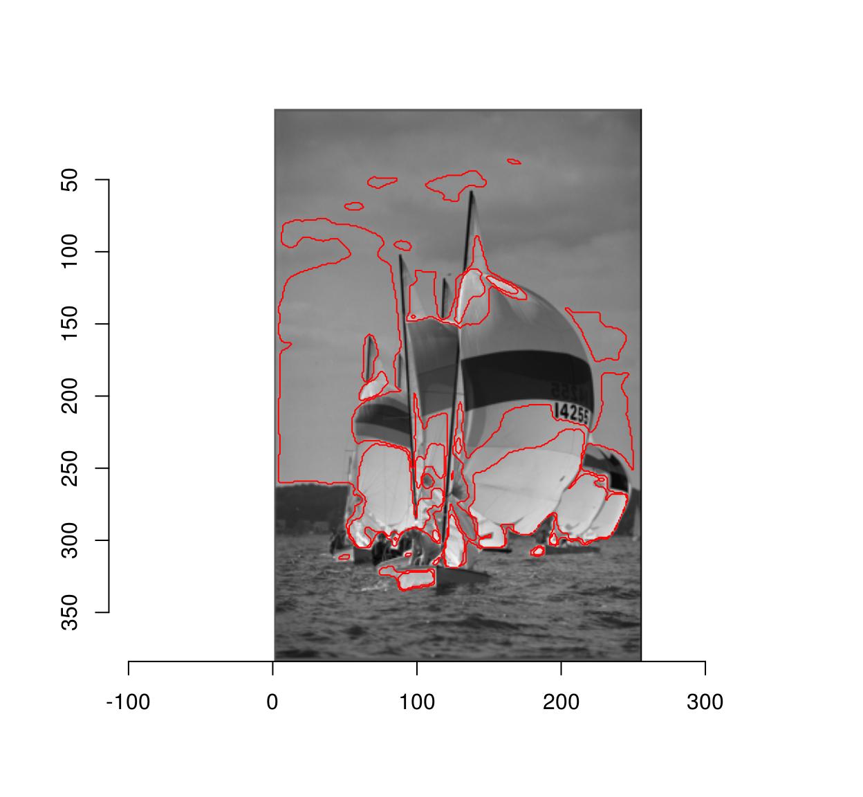
To select regions by colour similarity, the procedure is very similar, but we now need to compare values channel-by-channel and then sum:
#Select a colour on the red coat of the right-hand parrot
cl <- color.at(parrots,598,232)

#Produces an image of the same size as "parrots"
#filled with colour "cl"
cmp <- imfill(dim=dim(parrots),val=cl)

#Blur, compare, split across channels, compute Euclidean norm
d <- isoblur(parrots,2) %>% { . - cmp } %>% imsplit("c") %>% enorm
plot(d,main="Distance map")
points(598,232,col="red")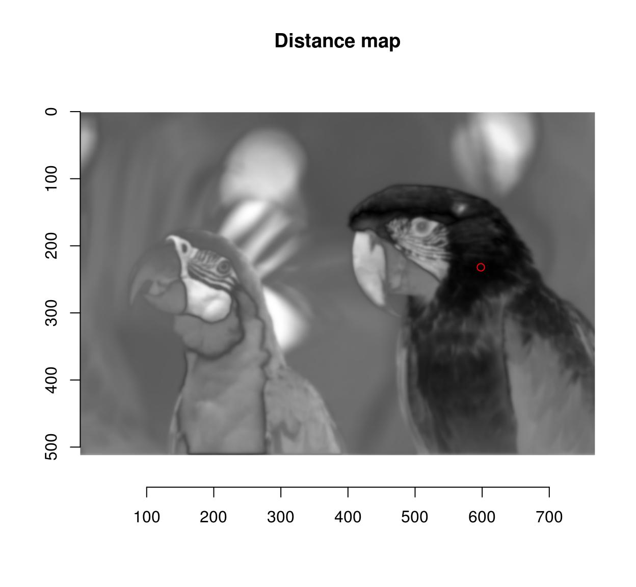
plot(parrots)
#Select 10% most similar pixels
(!threshold(d,"10%")) %>% highlight(col="black")
Here’s a function that does all this:
selectSimilar <- function(im,cl,thr="auto",sigma=2)
    {
        d <- isoblur(im,sigma) %>% { . - imfill(dim=dim(im),val=cl) } %>% imsplit("c") %>% enorm
        !threshold(d,thr)
    }
plot(parrots)
selectSimilar(parrots,cl,thr="10%",sigma=5) %>% highlight(col="blue")
Since the selection is by similarity of colour, CIELab space is more appropriate:
plot(parrots)
sRGBtoLab(parrots) %>%
    selectSimilar(color.at(.,330,457),thr="3%",sigma=2) %>%
    highlight(col="green")

parrots %>%
    selectSimilar(color.at(.,330,457),thr="3%",sigma=2) %>%
    highlight(col="red")
1.6 Magic scissors
This one does something fairly sophisticated and is left as an exercise to the reader. Roughly speaking, the idea is to find a path from point A to point B that’s orthogonal at every point to the gradient of the image. Here’s something to get you started, using the igraph package (which I don’t know all that well, which is why this bit of code can certainly be improved on). We convert the image to an adjacency graph, where each pixel is a node and there are edges between adjacent pixels. The edge weight is the difference in pixel values.
library(purrr)
library(igraph)

                                        #im <- grayscale(boats) %>% imresize(.5) %>% crop.borders(2)
im <- grayscale(parrots) %>% imresize(.5) %>% crop.borders(2)
##The following function makes a data.frame of links between pixel (x,y) and pixel (x+dx,y+dy)
##I'm sure there's a better way of doing things
make.df <- function(dx,dy) (abs(im-imshift(im,dx,dy)))%>%
                               as.data.frame%>%
                               mutate(x.to=x-dx,y.to=y-dy,id.from=paste(x,y,sep=","),id.to=paste(x.to,y.to,sep=",")) %>%
                               dplyr::select(id.from,id.to,value) %>%
                               dplyr::rename(weight=value)

##Get all neighbours, convert data.frame to graph
G <- cross2(-1:1,-1:1,function(a,b) abs(a) +abs(b) == 0) %>%
    map_df(lift(function(dx,dy) mutate(make.df(dx,dy),dx=dx,dy=dy))) %>%
    graph_from_data_frame

#Extract shortest from x=10,y=180 to x=120,y=100, convert back to coordinates
path <- shortest_paths(G,"10,180","120,100") %$% V(G)[vpath[[1]]]%>%
    names %>% stringr::str_split(",") %>%
    map_df(~ data.frame(x=as.integer(.[[1]]),y=as.integer(.[[2]])))

plot(im)
lines(path$x,path$y,col="red",lty=2,lwd=2)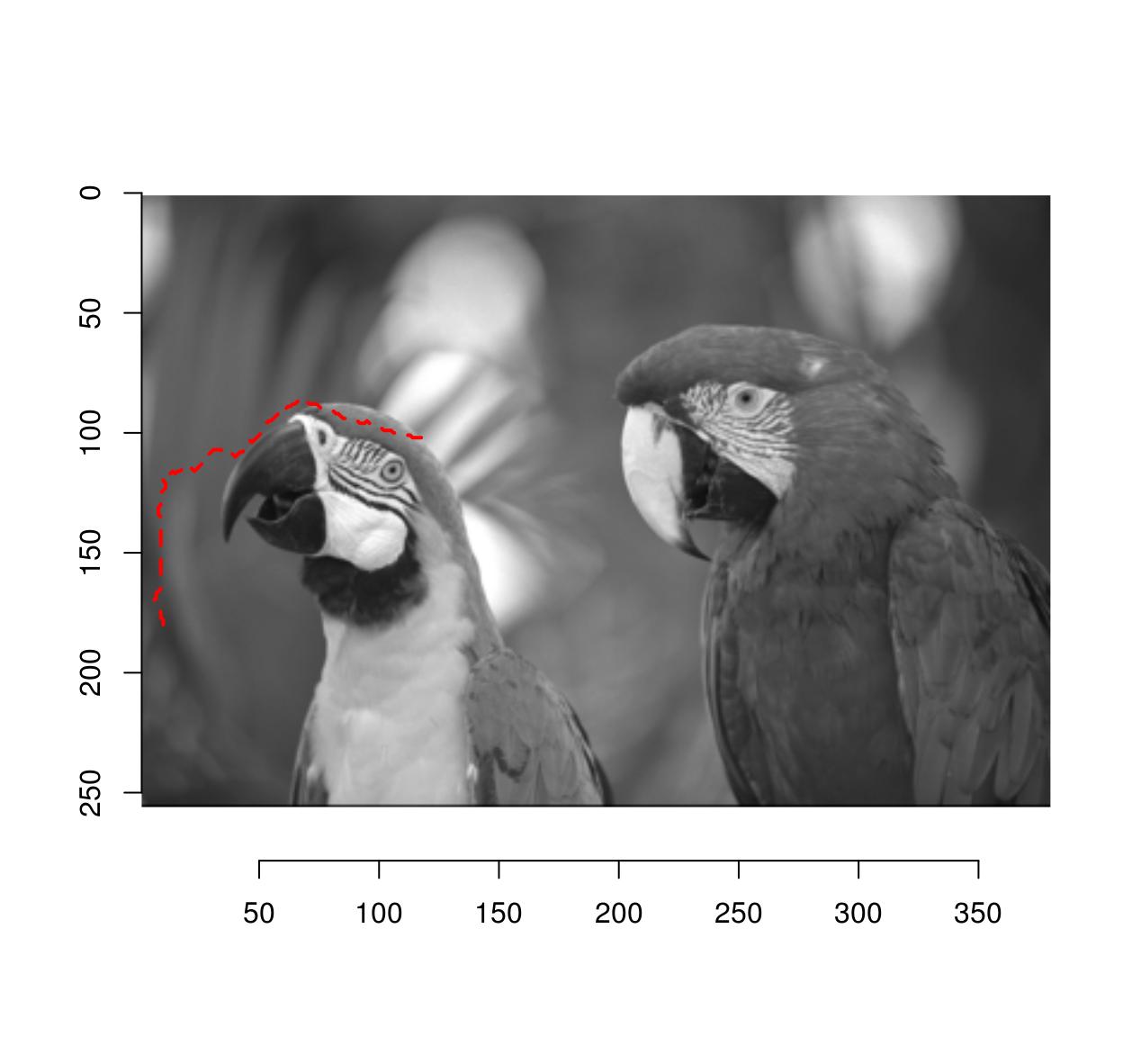
Notice how the path follows image regions of similar grayscale value.
1.7 Fuzzy selection (magic wand)
Flood selection selects all similar pixels around an initial point:
plot(parrots)
px.flood(parrots,100,100,sigma=.1) %>% highlight
#Higher tolerance
px.flood(parrots,100,100,sigma=.14) %>% highlight(col="darkred")
#Different initial point
px.flood(parrots,300,100,sigma=.1) %>% highlight(col="blue")
2 Drawing (paint tools)
2.1 Curves, text, etc.
To draw stuff on an image you can use the base R plotting tools along with “implot”. implot uses the image as canvas for an R plot, and returns an image. You only need to provide a piece of code that plots whatever you’d like to plot. Note that the coordinate system is the default one for images, i.e. (1…width)x(1…height).
#Let's add some text
parrots.mod <- implot(parrots,{ text(100,100,"ABCDEF",cex=4,col="red") })
plot(parrots.mod)
#Let's plot some random data
implot(parrots.mod,
{ points(width(parrots)*runif(50),height(parrots)*runif(50),col="darkblue",pch=24) }) %>%
    plot
2.2 Blur & sharpen
Whole-image blurs and sharpens are very easy to do:
isoblur(parrots,3) %>% plot
imsharpen(parrots,2) %>% plot
In the Gimp, the blur and sharpen tools allow you to blur and sharpen image regions selectively. In imager, you can do the same thing using masks:
#Select image region to blur
px <- px.flood(parrots,200,300,sigma=.58)
plot(parrots);highlight(px)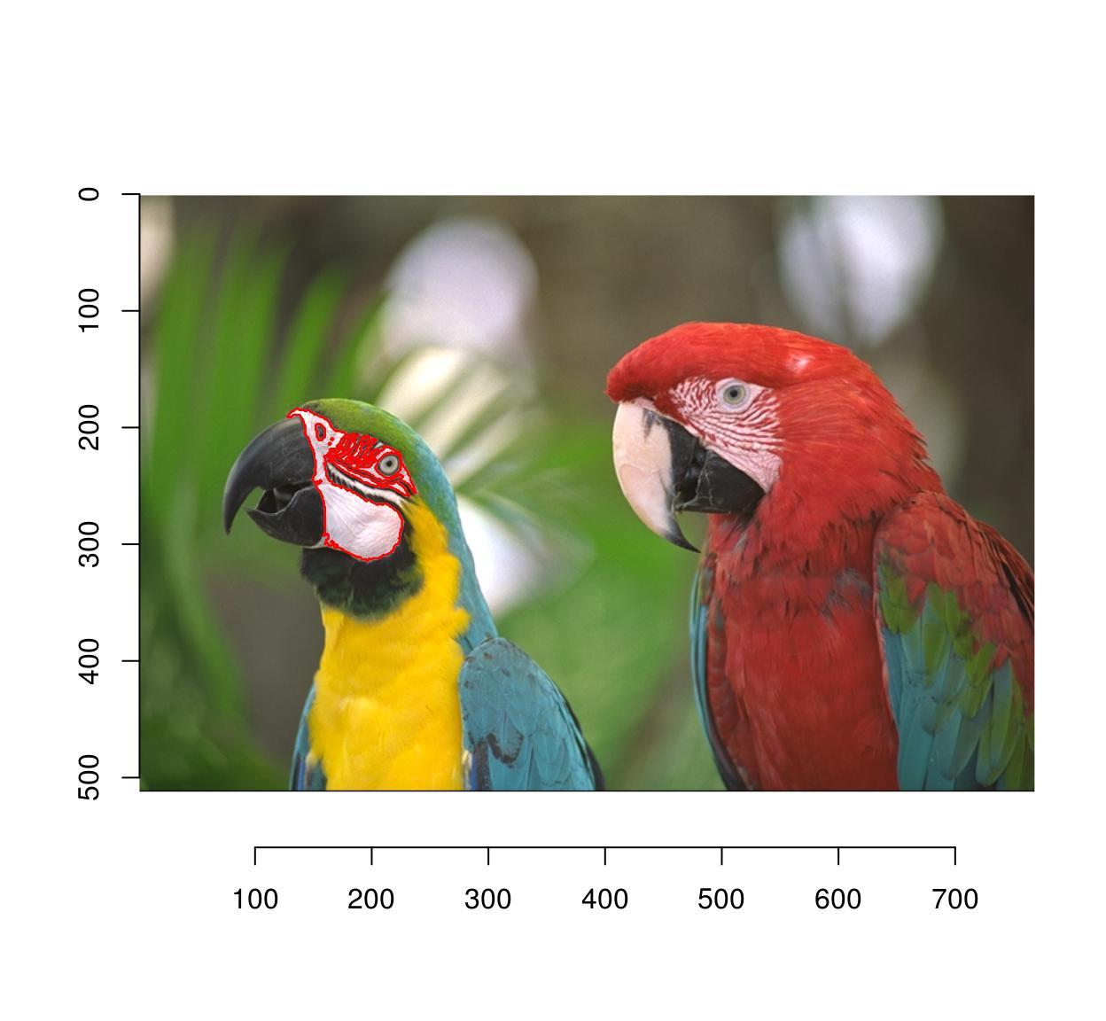
b <- isoblur(parrots,5)
msk <- as.cimg(px)
#Use mask to combine the blurred and original images
plot(parrots*(1-msk)+b*(msk))
2.3 Eraser
Pixsets!
#Erase the first 50 columns
px <- Xc(parrots) <= 50
im <- parrots
im[px] <- 0
plot(im)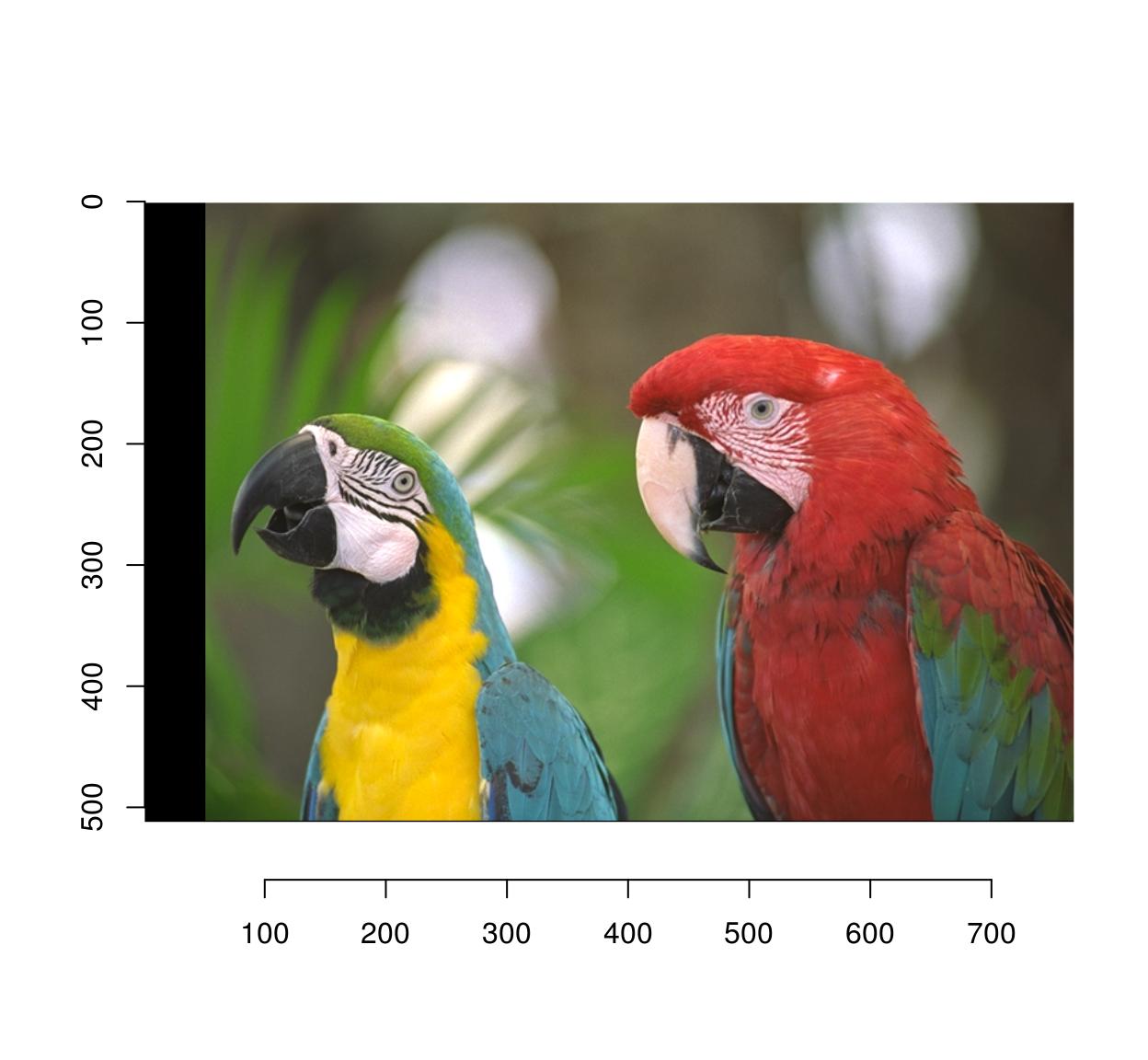
If instead of black, you need to fill in a different colour, use this:
im <- parrots
#make a uniform image of the same dimensions
#using a background colour of R=1,G=1,B=0 (yellow)
bg <- imfill(dim=dim(parrots),val=c(1,1,0))
msk <- as.cimg(px)
plot(bg*msk+(1-msk)*im)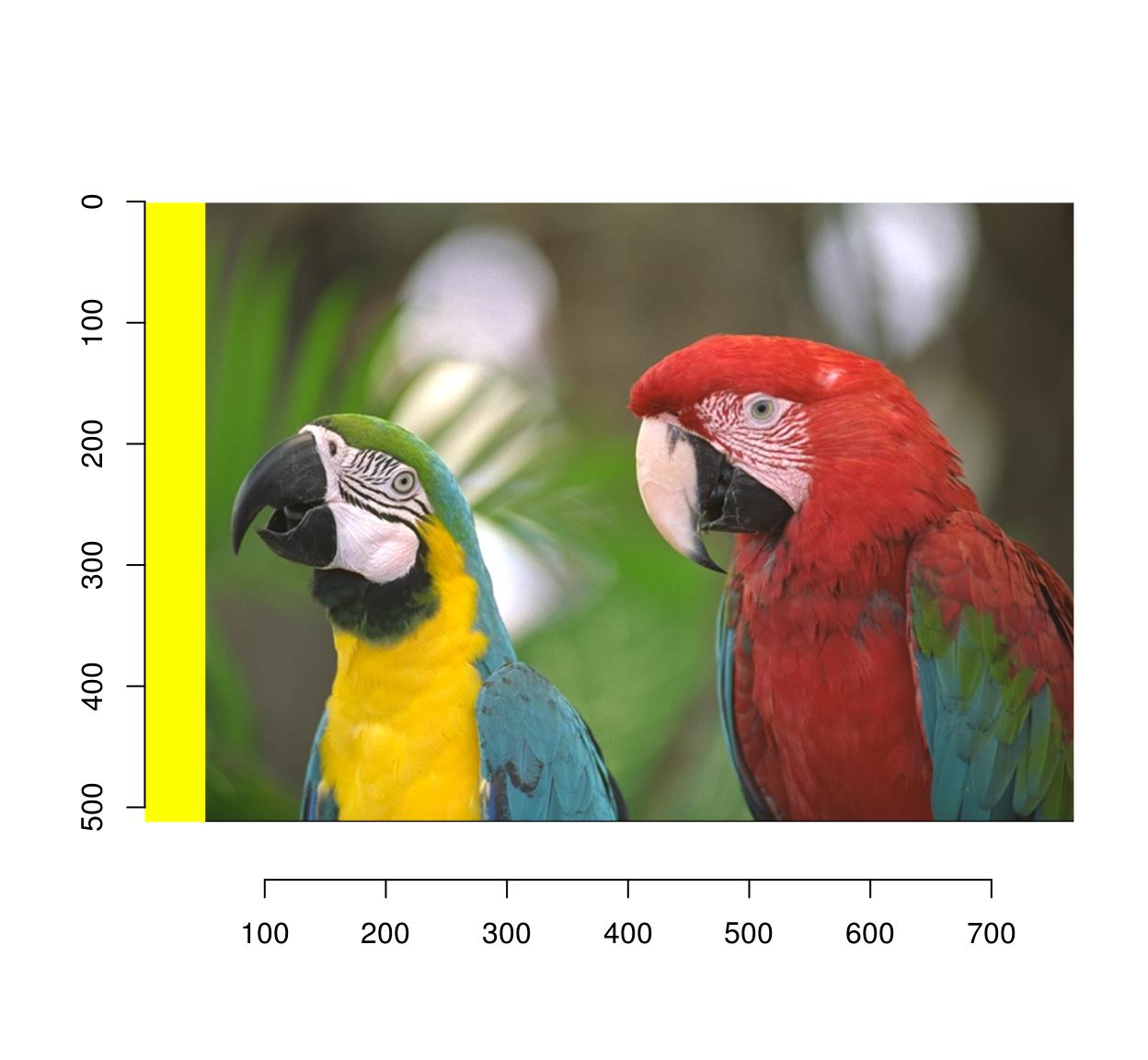
2.4 Smudge/dodge/burn/perspective clone etc.
I really doubt you need these ones. They’re fun exercises, though.
3 Transformations
3.1 Moving things about
Use imshift:
imshift(parrots,20,20) %>% plot
3.2 Rotations
Use imrotate:
imrotate(parrots,35,interp=2) %>% plot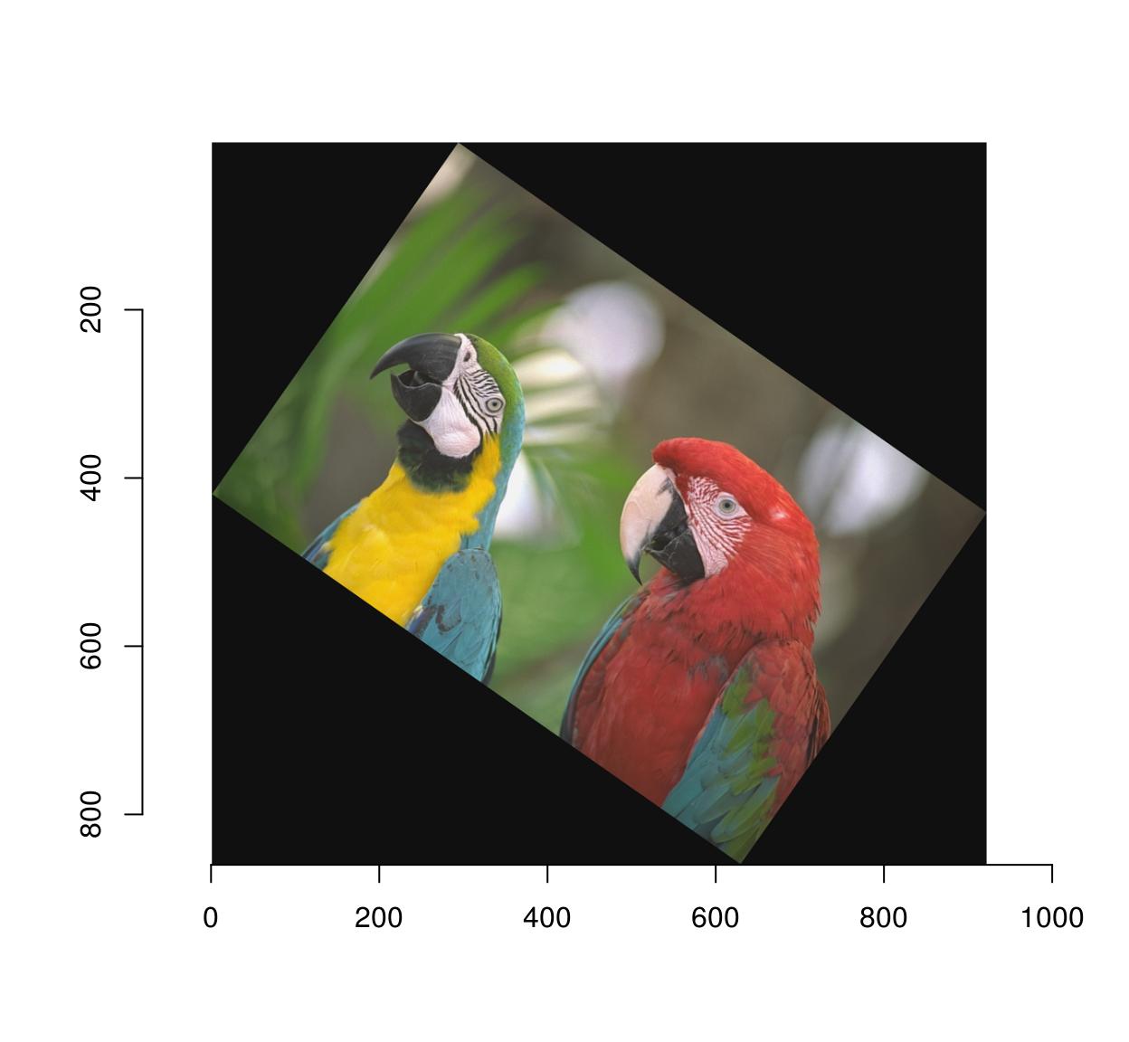
If you wish to shift the center of rotation, use the cx, cy arguments:
imrotate(parrots,35,cx=20,cy=20) %>% plot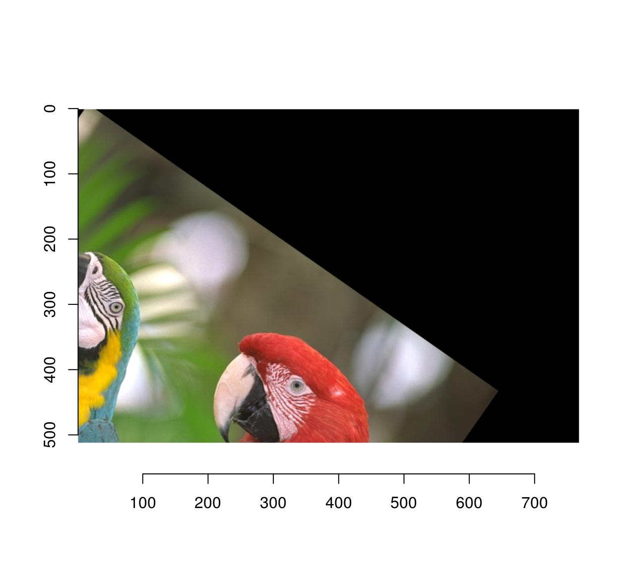
4 Scaling
Use imresize:
#Make a smaller copy of the image and append it:
imlist(parrots,imresize(parrots,.5)) %>%
    imappend("x") %>% plot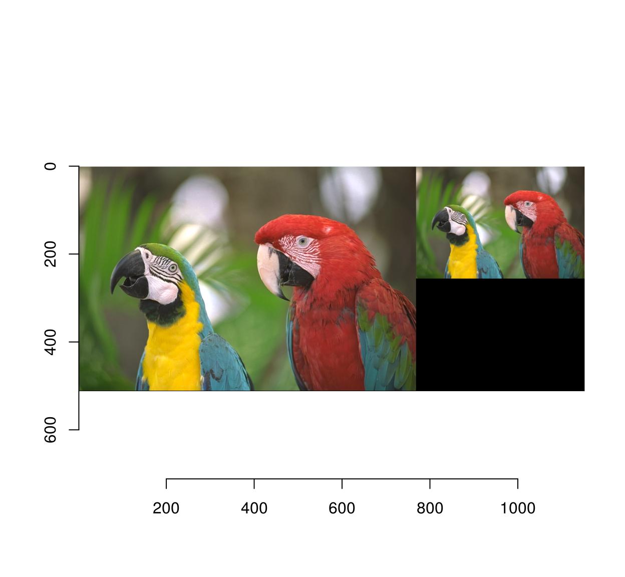
4.1 Flipping
mirror is your friend:
mirror(parrots,"x") %>% plot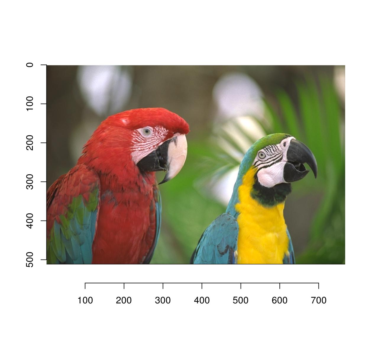
4.2 Cropping
Use imsub (see above) for general cropping. autocrop is another valuable tool which crops the outer parts of an image automatically:
#Define a mask from a pixset
msk <- px.flood(parrots,100,100,sigma=.28) %>% as.cimg
plot(parrots*msk)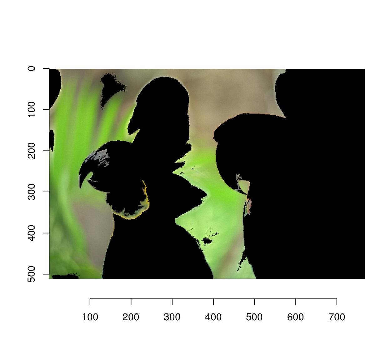
#Use autocrop to get rid of extra space
autocrop(parrots*msk) %>% plot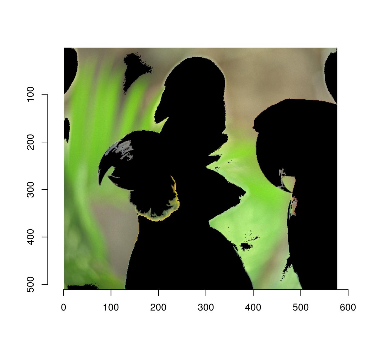
4.3 Shift, shear and other spatial transformations
General spatial transformations can be implemented via warping. Image warping consists in remapping pixels, ie. you define a function \(M(x,y)\) that displaces pixel content from position \(x,y\) to position \(x',y'\). For example, here’s a shift:
#We define an affine map from x,y to x',y'
map.shift <- function(x,y) list(x=x+10,y=y+30)
#imwarp performs the mapping
imwarp(parrots,map=map.shift) %>% plot
And here’s a 45° rotation around the origin:
#angle (in radians)
theta <- pi/4
map.rot <- function(x,y) list(x=cos(theta)*x-sin(theta)*y,
                                         y=sin(theta)*x+cos(theta)*y)
imwarp(parrots,map=map.rot) %>% plot
Notice that the image looks a bit strange, and indeed if we zoom in we see that there are artifacts:
imwarp(parrots,map=map.rot) %>%
    imsub(x < 200,y< 200) %>% plot(interp=FALSE)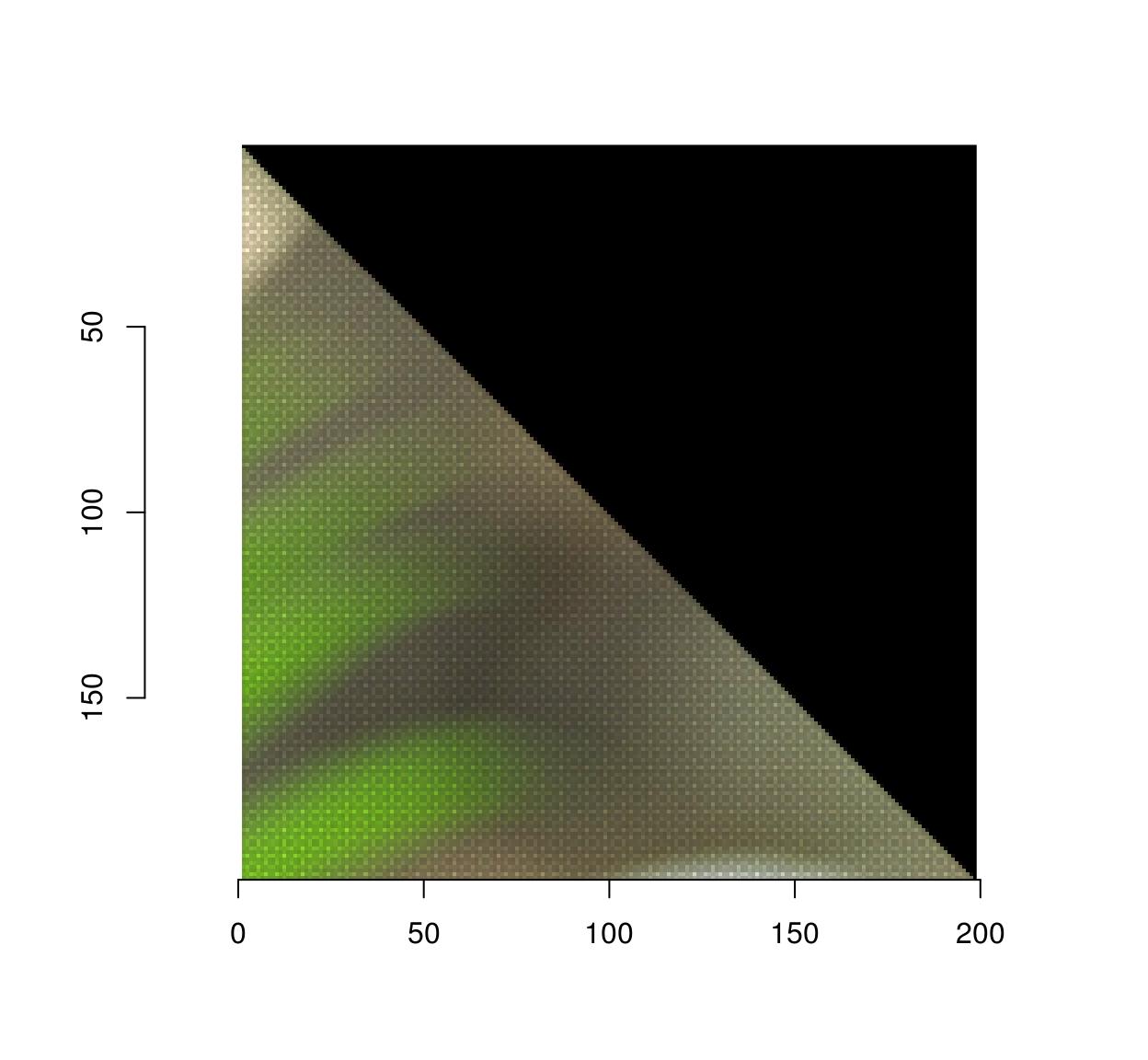
The reason this happens is that the algorithm works here in forward mode. Each pixel (x,y) is mapped to a new location (x’,y’) that may be off the image, or in between pixels, so the transformation can’t be computed exactly. The forward algorithm ends up painting in between pixels, which creates artifacts.
The backward algorithm involves specifying the inverse transformation, from (x’,y’) to (x,y).
#the inverse of the rotation above is another rotation
theta <- -pi/4
map.rot <- function(x,y) list(x=cos(theta)*x-sin(theta)*y,
                                         y=sin(theta)*x+cos(theta)*y)
imwarp(parrots,map=map.rot,direction="backward") %>% plot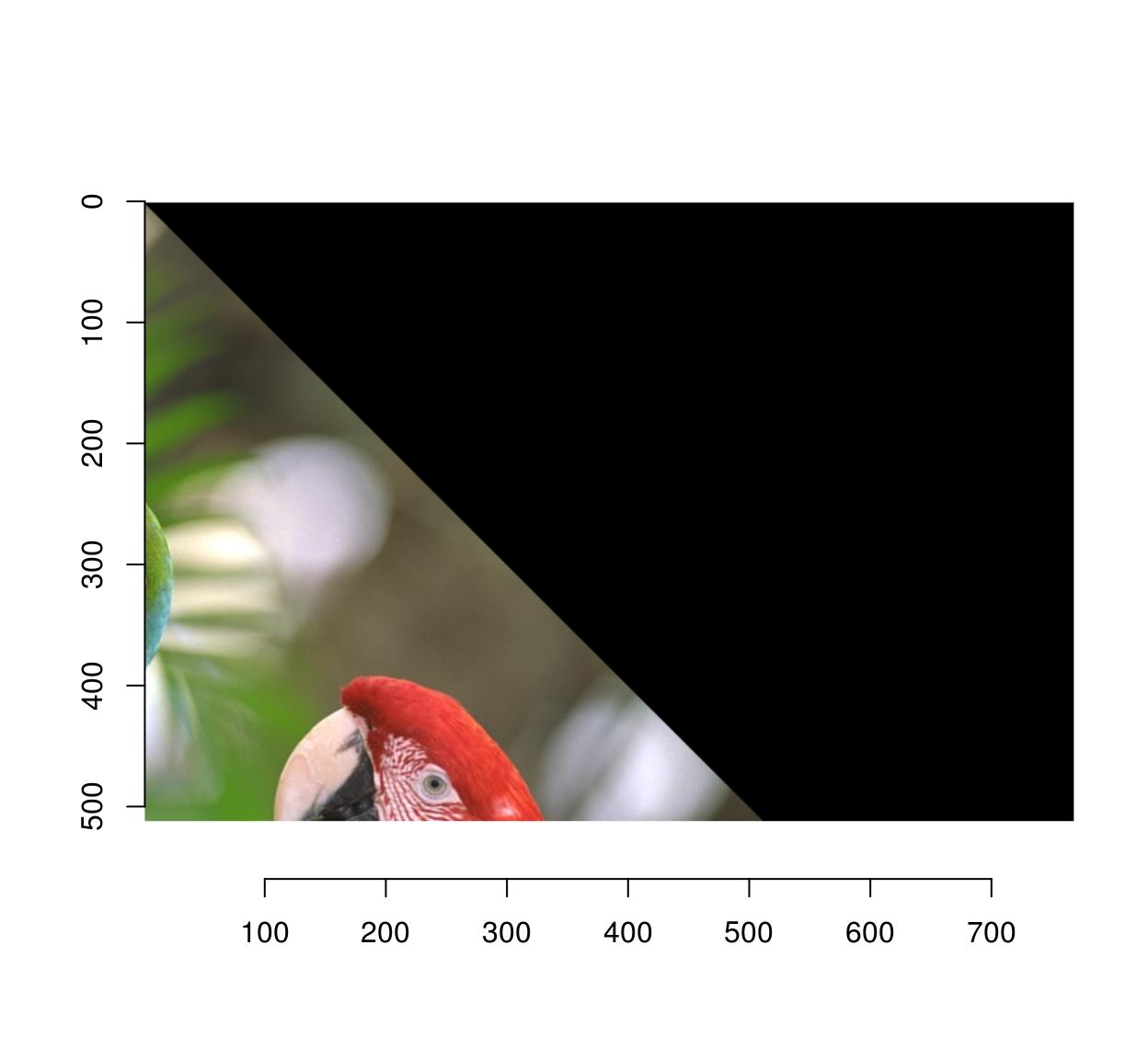
The artifacts are gone because the algorithm doesn’t have to paint in-between pixels anymore: if it needs to know the colour of pixel (x’,y’), it goes back to the original location (x,y) and interpolates.
Here’s a shear transformation:
map.shear <- function(x,y) list(x=x+.2*y,
                                    y=y)
imwarp(parrots,map=map.shear) %>% plot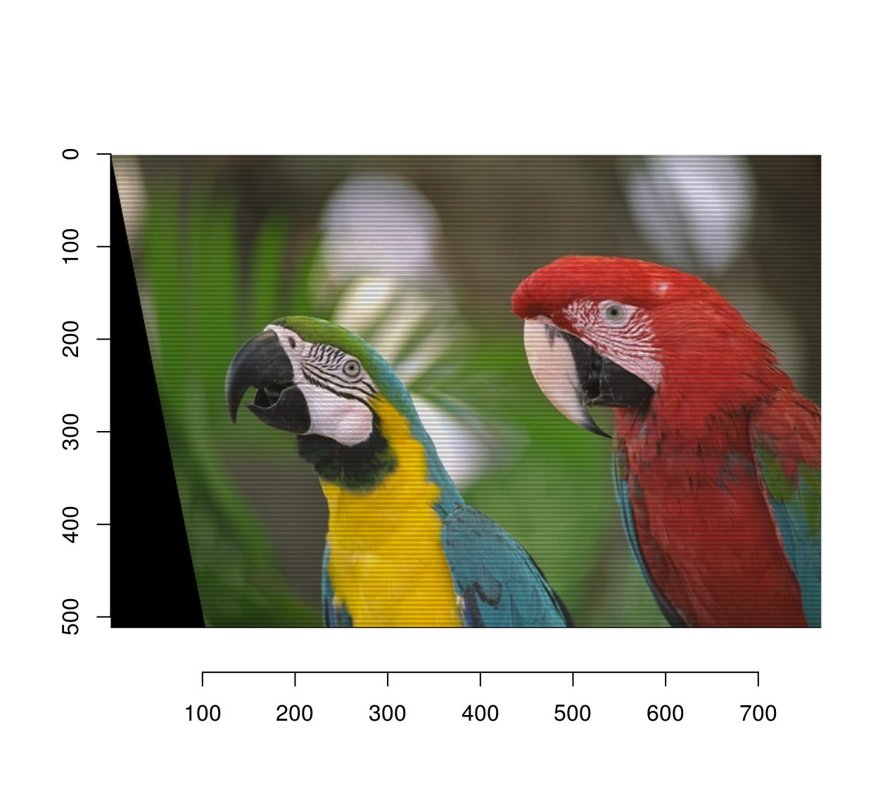
map.shear.rev <- function(x,y) list(x=x-.2*y,
                                    y=y)
imwarp(parrots,map=map.shear.rev,direction="backward") %>% plot
I’m leaving the perspective transform for the reader to figure out.